Workshop 4: The Tidy Data Mindset

Reshaping, Joining, and Tidying Clinical Data

Author

Your Name Here

Published

November 1, 2025

1. Introduction: What is “Tidy Data”?

In our previous sessions, we’ve been “wrangling” data. But what is our goal? The goal is to get our data into a “Tidy” format.

“Tidy Data” is a set of rules for organizing your data in R. If your data is “tidy,” all tidyverse packages (like dplyr and ggplot2) will work with it almost magically.

The rules are simple, but powerful:

Every column is a variable. (e.g., age, sbp, gender)
Every row is an observation. (e.g., one patient at one point in time)
Every cell is a single value.

This sounds obvious, but our clinical datasets are not currently tidy. Let’s see why and how to fix it.

First, let’s load our libraries and the three datasets we created.

library(tidyverse) # For data wrangling (dplyr, tidyr)
library(rio)       # For importing
library(here)      # For finding our files

# --- Load the Datasets ---
# We'll assume they are in a "data_raw" folder in our project

path_demo <- here("data_raw", "clinical_demographics.xlsx")
path_base <- here("data_raw", "clinical_baseline.xlsx")
path_fu   <- here("data_raw", "clinical_followup.xlsx")

df_demographics <- import(path_demo)
df_baseline     <- import(path_base)
df_followup     <- import(path_fu)

2. Combining Datasets: The Join Family

Right now, we have a problem. Our demographic data (like age and hypertension) is in one file, and our clinical data (like sbp and hba1c) is in another. We can’t analyze them together.

We need to join them. Joins combine two dataframes based on a shared “key” variable. In our case, the key is patient_id.

A left_join() keeps all rows from the left-hand data and matches what it can from the right-hand data.

This is the most common and safest join. Let’s join the baseline clinical data to our main demographics file.

# A left_join() keeps all rows from the "left" dataframe (x)
# and matches rows from the "right" dataframe (y).

# Let's see how many rows each has
nrow(df_demographics)

[1] 1000

nrow(df_baseline)

[1] 917

# We have 1000 demographic records, but only 917 baseline records.
# A left join will keep all 1000 demographic records.
# The 83 patients who don't have baseline data will get 'NA'
# for all the baseline columns.

df_full_baseline <- df_demographics |>
  left_join(df_baseline, by = "patient_id")

# View the result
glimpse(df_full_baseline)

Rows: 1,000
Columns: 13
$ patient_id              <chr> "PID_0001", "PID_0002", "PID_0003", "PID_0004"…
$ age                     <dbl> 66, 30, 54, 39, 65, 47, 53, 36, 65, 54, 66, 75…
$ gender                  <chr> "Female", "Male", "Female", "Female", "Male", …
$ tobacco_user            <chr> "No", "Yes", "No", "No", "Yes", "Yes", "No", "…
$ alcohol_user            <chr> "Yes", "Yes", "No", "No", "No", "No", "Yes", "…
$ physical_activity_level <chr> "Moderate", "Sedentary", "Moderate", "Moderate…
$ hypertension            <chr> "Yes", "Yes", "Yes", "Yes", "Yes", "Yes", "Yes…
$ diabetes                <chr> "Yes", "Yes", "No", "Yes", "Yes", "Yes", "No",…
$ weight_kg               <dbl> 72.87712, 82.65923, NA, 62.09445, 71.59333, 61…
$ height_cm               <dbl> 172.0, 176.0, 159.0, 156.5, 168.1, NA, 153.0, …
$ sbp                     <dbl> 153.4, 137.0, 139.6, 138.6, 130.0, 132.8, 152.…
$ dbp                     <dbl> 90.2, 89.0, 93.8, 84.8, 95.0, 81.4, 89.6, 84.2…
$ hba1c                   <dbl> 7.5, 7.5, 6.1, 6.7, 8.2, 9.2, 6.0, 8.3, NA, NA…

cat("Total rows in joined data:", nrow(df_full_baseline))

Total rows in joined data: 1000

An inner_join() keeps only the rows that exist in both datasets.

This is useful for finding the “intersection” of your data. It will only give us the 917 patients who appear in both df_demographics and df_baseline.

# An inner_join() only keeps rows that have a match in both dataframes.
df_inner <- df_demographics |>
  inner_join(df_baseline, by = "patient_id")

# View the result
glimpse(df_inner)

Rows: 917
Columns: 13
$ patient_id              <chr> "PID_0001", "PID_0002", "PID_0003", "PID_0004"…
$ age                     <dbl> 66, 30, 54, 39, 65, 47, 53, 36, 54, 66, 75, 49…
$ gender                  <chr> "Female", "Male", "Female", "Female", "Male", …
$ tobacco_user            <chr> "No", "Yes", "No", "No", "Yes", "Yes", "No", "…
$ alcohol_user            <chr> "Yes", "Yes", "No", "No", "No", "No", "Yes", "…
$ physical_activity_level <chr> "Moderate", "Sedentary", "Moderate", "Moderate…
$ hypertension            <chr> "Yes", "Yes", "Yes", "Yes", "Yes", "Yes", "Yes…
$ diabetes                <chr> "Yes", "Yes", "No", "Yes", "Yes", "Yes", "No",…
$ weight_kg               <dbl> 72.87712, 82.65923, NA, 62.09445, 71.59333, 61…
$ height_cm               <dbl> 172.0, 176.0, 159.0, 156.5, 168.1, NA, 153.0, …
$ sbp                     <dbl> 153.4, 137.0, 139.6, 138.6, 130.0, 132.8, 152.…
$ dbp                     <dbl> 90.2, 89.0, 93.8, 84.8, 95.0, 81.4, 89.6, 84.2…
$ hba1c                   <dbl> 7.5, 7.5, 6.1, 6.7, 8.2, 9.2, 6.0, 8.3, NA, 9.…

cat("Total rows in joined data:", nrow(df_inner))

Total rows in joined data: 917

A full_join() keeps all rows from both datasets. It’s the “union” of both.

This is less common, but useful if you have non-matching rows in both tables that you want to preserve.

# A full_join() keeps all rows from both X and Y.
# Since all baseline IDs are in demographics,
# this will give the same result as our left_join.
df_full <- df_demographics |>
  full_join(df_baseline, by = "patient_id")

cat("Total rows in joined data:", nrow(df_full))

Total rows in joined data: 1000

3. Reshaping Data: From “Wide” to “Long”

We have another problem. Our df_baseline and df_followup data is in two separate files. This is a very common “wide” data format.

df_baseline represents the “Time 0” observation.
df_followup represents the “Time 1” observation.

This violates our Tidy Data rules! * Rule 1 (Col is Variable): Is “Time” a variable? Yes! But right now, it’s split across two different dataframes. * Rule 2 (Row is Observation): Our unit of observation is patient + time.

We need to reshape this data. The goal is to have a single dataframe where we have new columns: 1. time_point (with values “Baseline” and “Followup”) 2. sbp, dbp, hba1c, etc., with the values for that time point.

Step 1: Add an ID to each dataframe

First, let’s add a time_point column to each file before we stick them together.

df_baseline_tagged <- df_baseline |>
  mutate(time_point = "Baseline")

df_followup_tagged <- df_followup |>
  mutate(time_point = "Followup")

Step 2: Combine with `bind_rows()`

Now that they have the exact same columns (including our new time_point column), we can stack them on top of each other using bind_rows().

# bind_rows() is the tidyverse way of stacking dataframes
df_long_clinical <- bind_rows(df_baseline_tagged, df_followup_tagged)

# Let's look at the result for one patient
df_long_clinical |>
  filter(patient_id == "PID_0001") # Note: This patient might not exist

  patient_id weight_kg height_cm      sbp      dbp    hba1c time_point
1   PID_0001  72.87712       172 153.4000 90.20000 7.500000   Baseline
2   PID_0001  73.19317       172 151.4024 79.81764 3.376654   Followup

Note: The patient might have NA for one time point if they were lost to follow-up!

Step 3: Join with Demographics

Now we have one “long” clinical dataframe and one demographic dataframe. We can join them!

df_analysis_ready <- df_demographics |>
  # We use an inner join to keep only patients with clinical data
  inner_join(df_long_clinical, by = "patient_id")

glimpse(df_analysis_ready)

Rows: 1,740
Columns: 14
$ patient_id              <chr> "PID_0001", "PID_0001", "PID_0002", "PID_0002"…
$ age                     <dbl> 66, 66, 30, 30, 54, 54, 39, 39, 65, 65, 47, 47…
$ gender                  <chr> "Female", "Female", "Male", "Male", "Female", …
$ tobacco_user            <chr> "No", "No", "Yes", "Yes", "No", "No", "No", "N…
$ alcohol_user            <chr> "Yes", "Yes", "Yes", "Yes", "No", "No", "No", …
$ physical_activity_level <chr> "Moderate", "Moderate", "Sedentary", "Sedentar…
$ hypertension            <chr> "Yes", "Yes", "Yes", "Yes", "Yes", "Yes", "Yes…
$ diabetes                <chr> "Yes", "Yes", "Yes", "Yes", "No", "No", "Yes",…
$ weight_kg               <dbl> 72.87712, 73.19317, 82.65923, 81.91229, NA, NA…
$ height_cm               <dbl> 172.0, 172.0, 176.0, 176.0, 159.0, 159.0, 156.…
$ sbp                     <dbl> 153.4000, 151.4024, 137.0000, 129.7916, 139.60…
$ dbp                     <dbl> 90.20000, 79.81764, 89.00000, 87.86196, 93.800…
$ hba1c                   <dbl> 7.500000, 3.376654, 7.500000, 3.307146, 6.1000…
$ time_point              <chr> "Baseline", "Followup", "Baseline", "Followup"…

This df_analysis_ready is now TIDY! 1. Columns are variables: patient_id, age, gender, … time_point, sbp, dbp… 2. Rows are observations: Each row is one patient at one time point.

Why is Tidy better?

Because analysis and plotting become incredibly simple.

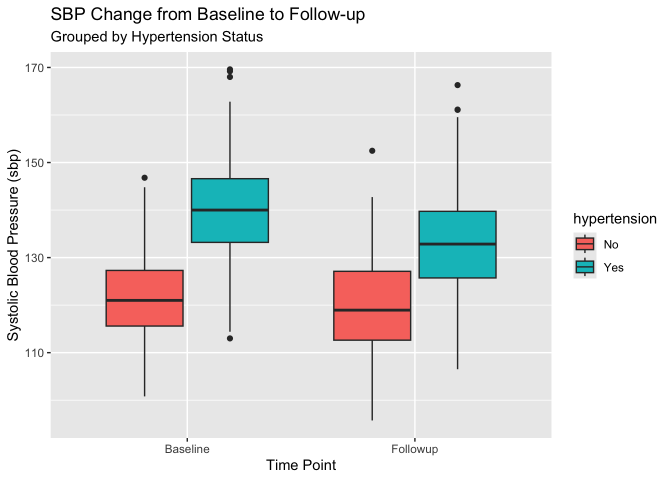
Question: How does average SBP change between Baseline and Followup, split by Hypertension status?

With our new tidy data, this is a simple group_by():

# We must first clean up NAs
df_analysis_ready |>
  filter(!is.na(sbp), !is.na(hypertension)) |>
  
  # Now the analysis is simple!
  group_by(hypertension, time_point) |>
  summarise(
    n_patients = n_distinct(patient_id), # count unique patients
    mean_sbp = mean(sbp),
    sd_sbp = sd(sbp)
  )

`summarise()` has grouped output by 'hypertension'. You can override using the
`.groups` argument.

# A tibble: 4 × 5
# Groups:   hypertension [2]
  hypertension time_point n_patients mean_sbp sd_sbp
  <chr>        <chr>           <int>    <dbl>  <dbl>
1 No           Baseline          203     122.   8.84
2 No           Followup          169     120.  10.1 
3 Yes          Baseline          687     140.   9.71
4 Yes          Followup          599     133.  10.3

With ggplot2, it’s just as easy. time_point and hypertension are just variables we can map.

df_analysis_ready |>
  filter(!is.na(sbp), !is.na(hypertension)) |>
  ggplot(aes(x = time_point, y = sbp, fill = hypertension)) +
  geom_boxplot() +
  labs(
    title = "SBP Change from Baseline to Follow-up",
    subtitle = "Grouped by Hypertension Status",
    x = "Time Point",
    y = "Systolic Blood Pressure (sbp)"
  )

4. The Other Way: `pivot_wider()`

Sometimes, you get data that is too long. This is common in survey data or lab data, where you have one row per lab test.

Let’s imagine our df_long_clinical data was even “longer”:

# Let's just use a few columns for this example
df_longer_example <- df_long_clinical |>
  select(patient_id, time_point, sbp, dbp, hba1c) |>
  # pivot_longer() is the master function for this
  pivot_longer(
    cols = c(sbp, dbp, hba1c), # Columns to stack
    names_to = "measurement_type", # New column for the *name*
    values_to = "value"            # New column for the *value*
  )

glimpse(df_longer_example)

Rows: 5,220
Columns: 4
$ patient_id       <chr> "PID_0676", "PID_0676", "PID_0676", "PID_0016", "PID_…
$ time_point       <chr> "Baseline", "Baseline", "Baseline", "Baseline", "Base…
$ measurement_type <chr> "sbp", "dbp", "hba1c", "sbp", "dbp", "hba1c", "sbp", …
$ value            <dbl> 131.6, 78.8, 6.5, 145.0, 91.0, 9.3, 136.4, 90.2, 7.7,…

This is also tidy! But it’s not always what you want. What if you want to create a sbp_change variable? You’d have to filter, join, and subtract.

It’s often easier to have sbp_baseline and sbp_followup in the same row. We can use pivot_wider() to do this.

pivot_wider() is the opposite of pivot_longer(). It takes a “long” dataset and spreads it out into a “wide” one.

# Let's take our analysis-ready data
df_analysis_ready |>
  select(patient_id, time_point, sbp, dbp, hba1c) |>
  
  pivot_wider(
    # The new column *names* will come from the 'time_point' column
    names_from = time_point,
    
    # The *values* for those new columns will come from sbp, dbp, hba1c
    values_from = c(sbp, dbp, hba1c)
  )

# A tibble: 917 × 7
   patient_id sbp_Baseline sbp_Followup dbp_Baseline dbp_Followup hba1c_Baseline
   <chr>             <dbl>        <dbl>        <dbl>        <dbl>          <dbl>
 1 PID_0001           153.         151.         90.2         79.8            7.5
 2 PID_0002           137          130.         89           87.9            7.5
 3 PID_0003           140.         131.         93.8         93.4            6.1
 4 PID_0004           139.         131.         84.8         84.4            6.7
 5 PID_0005           130          135.         95           94.1            8.2
 6 PID_0006           133.         127.         81.4         74.8            9.2
 7 PID_0007           152.         148.         89.6         94.7            6  
 8 PID_0008           139.         130.         84.2         78.1            8.3
 9 PID_0010           135.         120.         93.8         84.9           NA  
10 PID_0011           145.         145.         86.2         79.3            9  
# ℹ 907 more rows
# ℹ 1 more variable: hba1c_Followup <dbl>

Look at the column names! We now have sbp_Baseline, sbp_Followup, dbp_Baseline, etc. This is a “wide” format, but it’s very useful for calculating change scores.

df_wide_analysis <- df_analysis_ready |>
  select(patient_id, age, gender, hypertension, time_point, sbp) |>
  pivot_wider(
    names_from = time_point,
    values_from = sbp
  ) |>
  # Now we can easily calculate change!
  # (Make sure to handle NAs)
  mutate(
    sbp_change = Followup - Baseline
  )

glimpse(df_wide_analysis)

Rows: 917
Columns: 7
$ patient_id   <chr> "PID_0001", "PID_0002", "PID_0003", "PID_0004", "PID_0005…
$ age          <dbl> 66, 30, 54, 39, 65, 47, 53, 36, 54, 66, 75, 49, 55, 70, 5…
$ gender       <chr> "Female", "Male", "Female", "Female", "Male", "Female", "…
$ hypertension <chr> "Yes", "Yes", "Yes", "Yes", "Yes", "Yes", "Yes", "Yes", "…
$ Baseline     <dbl> 153.4, 137.0, 139.6, 138.6, 130.0, 132.8, 152.2, 139.4, 1…
$ Followup     <dbl> 151.4024, 129.7916, 130.5179, 130.8764, 135.1710, 127.087…
$ sbp_change   <dbl> -1.99764019, -7.20843049, -9.08205892, -7.72364909, 5.171…

# Now we can analyze the *change*
df_wide_analysis |>
  filter(!is.na(sbp_change), !is.na(hypertension)) |>
  group_by(hypertension) |>
  summarise(
    mean_sbp_change = mean(sbp_change)
  )

# A tibble: 2 × 2
  hypertension mean_sbp_change
  <chr>                  <dbl>
1 No                     -1.93
2 Yes                    -6.99

Summary

Tidy Data: Columns = Variables, Rows = Observations.
Joins: Combine datasets.
- left_join(): Keeps all from the left. (Most common)
- inner_join(): Keeps only matching rows.
Pivoting: Reshaping your data.
- bind_rows(): Stacks two dataframes.
- pivot_longer(): Makes “wide” data “long”.
- pivot_wider(): Makes “long” data “wide”.